Table of contents
Introduction
Autoencoders are a fascinating approach to unsupervised learning, especially notable for their diverse applications. This project highlights three significant applications:
Dimensionality Reduction: Demonstrates how an alphabet of 35 pixel letters can be represented through a 2-dimensional space, effectively reducing the manifold of 35 variables (the input) to a 2-variable manifold, facilitating dimensionality reduction.
Denoising: Illustrating that after training a denoising autoencoder to reproduce input without noise, it can process noisy letter and output the original letter.
Generation: By adjusting the original autoencoder to create a continuous latent space, new emojis that the model wasn't explicitly trained on can be generated.
Autoencoder
The goal of an autoencoder is to compress (encode) the input into a lower-dimensional latent space and then reconstruct (decode) the output from this representation. The process aims to capture the most relevant aspects of the data necessary to reconstruct the input as closely as possible.
An autoencoder consists of two main components: the encoder and the decoder. The encoder maps the input to the latent space (encoding), and the decoder attempts to generate the original input from the latent space representation.

Mathematically, for an input vector x in Rn, the encoder function f(x) maps x to a latent representation z in Rm where m < n. The decoder function g(z) then maps z back to the reconstruction x' in Rn. The objective is to minimize the difference between x and x', often using the mean squared error (MSE):

It's interesting remarking than in itself the architecture is the same a Multi-layer Perceptron (MLP) architecture, with the disclaimer that expected is the same as the input. Because of this we do not labels (as a in a typical MLP training pipeline), and as such this architecture is unsupervised.
Results
In terms of result we managed to reduce the dimensionality of a 27-letter alphabet of 5x7 pixel characters into a 2 dimension latent space.
See Figure 3 for the output of the autoencoder for ever input. All letters are matched almost perfectly except for some that differ by a single character, for instance the letter i in the right corner.

Similarly, because the latent space is two dimensional we can plot it, see Figure 4. Interestingly, certain letters are closer between themselves for instance n/m and e/o.

Denoising Autoencoder - DAE
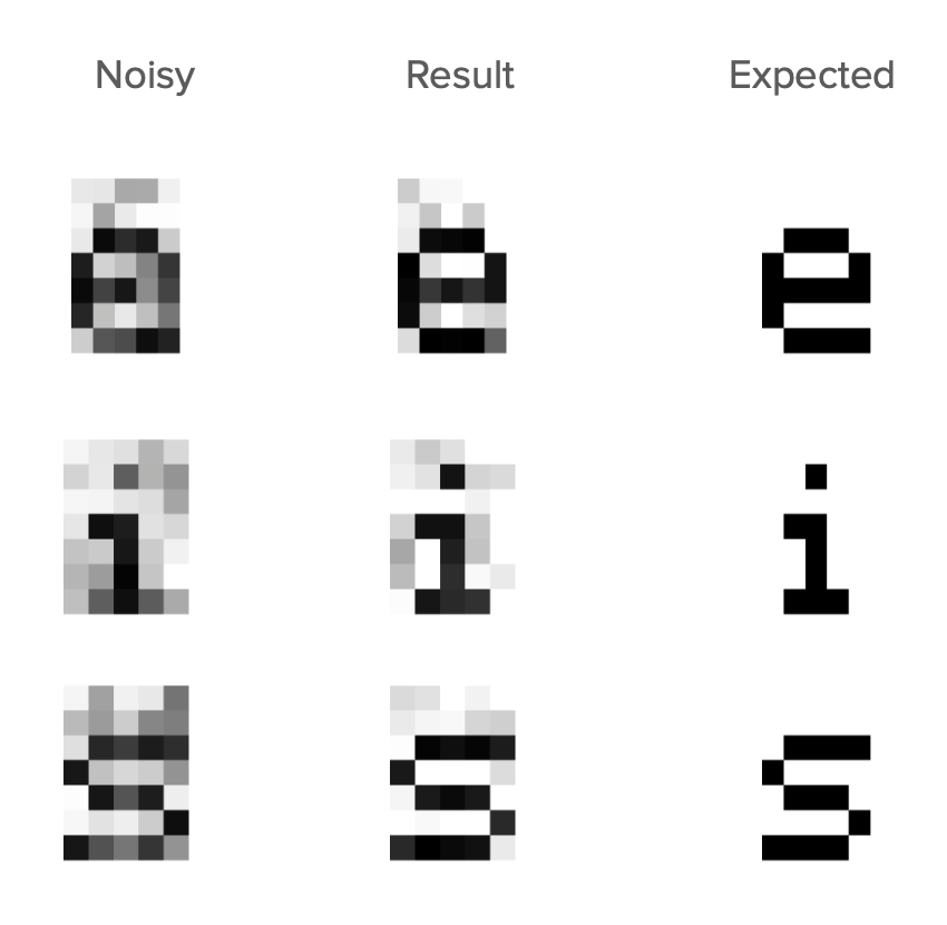
A denoising autoencoder aims to remove noise from the input data. It is trained to ignore the noise in the input and recover the original, undistorted input. The training involves adding noise to the input data, then training the autoencoder to reconstruct the original, noise-free data.
If x is the original input and x' is the noisy input, the encoder maps x' to a latent representation z, and the decoder reconstructs the noise-free input y from z. The loss function MSE is used to minimize the difference between the original clean data x and the reconstructed data y. In other words, it's the same architecture to the vanilla autoencoder, only the training changes.

We tested with numerous with two kind of noises:
- Salt and Pepper: is a form of noise in images where pixels are set to either the maximum value (which looks like salt in the image) or the minimum value (which looks like pepper)
- Gaussian: is a statistical noise having a probability density function equal to that of the normal distribution, also known as the Gaussian distribution. It is characterized by adding to each pixel value a random value chosen from a Gaussian distribution. This results in a more subtle form of noise compared to Salt and Pepper noise, often resembling a grainy appearance over the image.
Results
Salt and Pepper Noise
In Figure 6, the input images with Salt and Pepper noise display this characteristic scattering of white and black pixels. The DAE aims to filter out these disturbances, reconstructing images that closely resemble the clean, original images. The output images demonstrate the effectiveness of the DAE in removing this type of noise, restoring the image quality while maintaining the integrity of the original data.

Gaussian Noise
In Figure 7, the input images with Gaussian noise show this grainy, blurred effect across the entire image. The DAE's task is to identify and remove this noise, aiming to reconstruct images that are as close to the original, clean versions as possible. The output images illustrate the capability of the DAE to effectively mitigate the impact of Gaussian noise, enhancing the clarity and recognizability of the image details.
Variational Autoencoder - VAE
Variational Autoencoders (VAEs) are a sophisticated variant of standard autoencoders that introduce probabilistic interpretations and can generate new data points. Unlike traditional autoencoders, VAEs model the encoding as a continuos distribution over the latent space.
Architecture
VAEs assume that data is generated by a random process involving an unobserved continuous variable z. The encoder outputs a distribution over the latent space characterized by mean μ and variance σ2. We then use these mean and variance, in par with a random variable ε, to generate the latent space input to the generative network. This last step is the Reparametrization Trick, also applied beyond VAEs.
For a depiction of the VAE architecture see Figure 7.

In terms of the implementation, we initally tried building a single MLP for the vanilla autoencoder, but this architecture was not conducive to the VAE. Because the goal of the VAE was to generate new patterns, we broke the autoencoder into two MLP architectures, having thus the ability to decouple the recognition model from the generative model.
We also used a latent-space of two dimension, having the median and variance of each variable in our latent space defined by the recognition network (this was then used through the reparametrization trick to generate the continuos latent space.)
Loss Function
Whereas the previous autoencoder implementations had only one term to the loss function, the VAE has two. That is, in addition to the MSE it has a regularization term designed to achieve a better distribuition of the examples through the latent space.

Reconstruction Loss
This is identical to the other two autoencoders, it's what allows the architecture to learn to encode and decode the examples through the latent space.

KL-Divergence Loss
This is a measure of how the probability distribution over the latent variables z
, as modeled by the encoder, diverges from the prior distribution. The prior distribution being that of ε which is obtained from a normal distribution. As a result, this term of the loss function forces the distribuition of each example in the latent space to ressemble a normal distribution. It is used to regularize.

Backpropagation
It's worth noting that the MLP architecture we had previously defined had the backpropagation designed ad hoc, as a result we took the time to carefully figure out the partial derivates to be able to connect the gradient coming from the generative network to the gradient of the recognition network. We leave the derivatives to the reader, they are quite simple.

Results: Generation
We created a new dataset for this step, see Figure 12 for the emojis chosen for training. Also note we modified the input size as the emojis are 12x12 pixels.
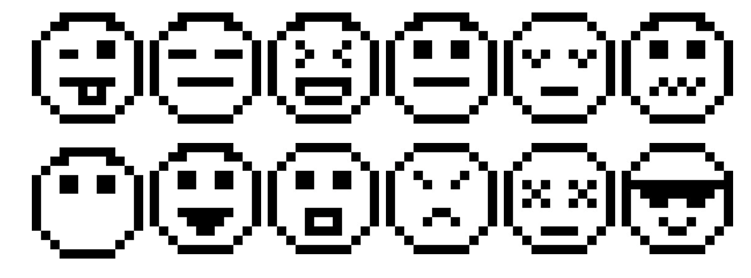
Once the VAE is trained, we detach the generator and generate images by just traversing the latent space at different intervals and saving the images generated by the model. See Figure 13 for the picture. It can be seen how the VAE generates different emojis for each vector in the latent-space, even generating emojis that were not previously seen in training.

Conclusion
In summary, autoencoders, with their simple yet powerful structure, offer a wide range of possibilities in unsupervised learning tasks. From compressing data to cleaning it and even generating new instances, autoencoders prove to be invaluable tools in the arsenal of machine learning practitioners. Moreover, although seemingly complex from the outset, they can be implemented from scratch.